Types of Microeconomics or Microeconomic Analysis

Types of Microeconomic Analysis

There are three types of microeconomic analysis or types of microeconomics categorized by time considerations. They are listed as follows:

Micro Statics or Micro Static Analysis,
Comparative Micro Statics or Comparative Micro Static Analysis, and
Micro Dynamics or Micro Dynamic Analysis.

Each of these types of Microeconomics is discussed in detail below:

1. Micro Statics or Micro Static Analysis

Micro statics is a branch of microeconomics that deals with the study of individual markets and the factors determining the equilibrium price and quantity in a market. This includes the study of supply and demand and the various factors that can affect the supply and demand for a good or service, such as changes in prices, incomes, or preferences.

Micro statics is often contrasted with microdynamics, which is a branch of microeconomics that deals with the study of how markets and economies change over time. This includes studying how individual markets adjust to changes in supply and demand and how these changes can affect the overall economy.

For example, let us consider a market for apples where the supply and demand are initially in equilibrium at a certain price. If the demand for apples suddenly increases, then this will create a state of disequilibrium in the market. The higher demand will cause the market price for apples to increase, which will, in turn, incentivize producers to increase their supply of apples to meet the higher demand and make a profit. As the supply increases to meet the higher demand, the market will eventually return to a state of static equilibrium at the new, higher price.

Different economists may have slightly different definitions of micro statics, but some common definitions of this field are as follows:

“An economy in which rates of output are constant is called static.” – Prof. Harrod

“Economic statics covers that part of economic theory where we do not trouble about dating.” – J.R. Hicks

Assumptions of Micro Statics:

Micro Static is a branch of economics that focuses on the study of equilibrium in markets and economies. This approach is based on a number of assumptions, which are simplifying assumptions that are made in order to make the analysis tractable and allow for useful conclusions to be drawn. Some of the critical assumptions of static economic analysis include the following:

Markets are in equilibrium: One of the critical assumptions of static analysis is that markets are in equilibrium. This means that the supply and demand for a good or service are balanced, resulting in a stable market price. This assumption allows for the study of the factors that determine the equilibrium price and quantity in a market.
Prices are flexible: Another assumption of static analysis is that prices are flexible and can adjust to changes in supply and demand. This means that if there is excess demand or excess supply in a market, the market price will change in order to bring supply and demand back into balance. This assumption is often justified by the idea that market participants will respond to changes in prices in order to maximize their own welfare.
Market participants are rational: Static analysis often assumes that market participants are rational, meaning that they make decisions based on their own self-interest. This means that they will respond to changes in prices, incomes, or preferences in a way that maximizes their own welfare. This assumption allows for the study of how market participants will respond to changes in the market.
Market participants have perfect information: Another assumption of static analysis is that market participants have perfect information. This means that they have complete and in-depth information regarding the market.

Diagram of Micro Statics

The concept of Micro statics can be clarified with the help of the following diagram:

The above figure shows prices and quantities on the Y and X axes, respectively. To determine the price OP and quantity OQ at a given time period, the demand curve (D) intersects the supply curve (S) at point E. Point E represents the static equilibrium. This analysis is a static equilibrium analysis.

2. Comparative Micro Statics or Comparative Micro Static Analysis

Comparative Micro Statics compares the equilibrium outcomes of two or more market situations. This entails examining the various factors that influence supply and demand and the resulting equilibrium price and quantity.

The comparative statics assessment is a crucial tool in Comparative Micro Statics. This usually involves comparing a market’s equilibrium outcome before and after a change in one or more of its underlying variables. For instance, an examination of a tax’s impact on a market’s equilibrium outcome.

We must first determine the market’s initial equilibrium outcome to conduct a comparative statics analysis. This can be done by analyzing the supply and demand curves and determining where they intersect. After determining the initial equilibrium outcome, we can introduce a change in one of the underlying variables, such as a tax on the market’s supply side.

We can determine the new equilibrium outcome by analyzing the new supply and demand curves that result from the change. By comparing the two equilibrium outcomes, we can see how the change affects the market and the behaviour of its participants.

According to Paul A. Samuelson, “Comparative Micro Statics refers to the study of economic phenomena at a particular point in time with a focus on comparing the conditions of one market with those of another market. It is concerned with the analysis of the behaviour of economic agents, such as consumers and firms, under different market structures.”

In the words of Lionel Robbins, “Comparative Micro Statics involves the comparison of two or more alternative hypothetical states of a given market situation, with the aim of studying the effects of changes in the variables that govern the market. It focuses on the analysis of the allocation of resources and the distribution of income under different market conditions.”

James Tobin defines Comparative Micro Statics as the study of the behaviour of individual economic agents, such as consumers, producers, and investors, in response to changes in prices, incomes, and other economic variables. It is concerned with the analysis of the factors that influence the demand and supply of goods and services in different markets and how these factors affect the allocation of resources and the distribution of income.

Diagram of Comparative Micro Statics

The concept of Comparative Micro statics can be clarified with the help of the following diagram:

The Y and X axes in the figure above represent prices and quantities, respectively. Due to a change in the variable of the demand function, the demand curve shifts from D to D₁, resulting in a new equilibrium at point F. At this point, the price is determined to be OP₁ and the quantity is OQ₁. The comparison of the values of the variables between the two equilibrium points, E and F, is known as Comparative Statics.

Features of Static Equilibrium:

In general, micro statics is characterized by the following properties:

Focus on individual markets: Micro statics focuses on the behaviour of individual markets rather than the overall economy. This means it examines the supply and demand for a specific good or service and the factors determining the equilibrium price and quantity in that market.
Use of supply and demand analysis: Micro statics uses supply and demand analysis to understand the behaviour of individual markets. This involves examining the factors that affect the supply and demand for a good or service and how these factors determine the equilibrium price and quantity in a market.
Static analysis: Micro statics is a static analysis, meaning that it focuses on the equilibrium state of a market at a given point in time rather than how the market changes over time. It does not consider how supply and demand may change in response to market or economic changes.
Emphasis on equilibrium: Micro statics strongly emphasizes the concept of equilibrium, which is a state of balance in which the supply and demand for a good or service are equal. This means that micro statics focuses on understanding how markets reach equilibrium and how the equilibrium price and quantity are determined.

Features of Static Equilibrium by J.B Clark

Some of the features of the Static economy pointed out by Professor Clark are enlisted as follows:

It focuses on the study of individual markets rather than the overall economy.
It concerns the equilibrium in a market rather than changes over time.
It examines the factors that determine the supply and demand for a good or service, such as prices, incomes, and preferences.
It uses the concept of equilibrium to explain the behaviour of individual markets.
It is based on the assumptions of rationality and profit maximization by market participants.
It is often contrasted with microdynamics, which focuses on studying changes in markets and economies over time.

These properties describe the focus and approach of micro-statics within the field of microeconomics.

Scopes and Importance of Static Economy:

In economics, static analysis is a method of studying the behaviour of an economy over a short period of time without considering changes over time. This approach is based on the assumption that the economy is in a state of equilibrium and that changes in the economy are small and do not significantly affect the equilibrium.

The scopes and importance of static analysis in economics are as follows:

It allows for the study of individual markets and the factors that determine a market’s equilibrium price and quantity. This can help to understand the behaviour of individual markets and the forces that shape market outcomes.
It provides a framework for analyzing the effects of supply and demand changes on a market’s equilibrium. This can help to understand how changes in the economy can affect market prices and quantities and how markets can adjust to these changes.
It can be used to analyze the effects of government policies on the economy, such as changes in taxes or subsidies. This can help to understand how these policies can affect the behaviour of individual markets and the overall economy.
It can be used to analyze the distribution of income and wealth in an economy and how changes in market prices can affect the distribution of income and wealth.
It can be used to analyze the efficiency of an economy and how changes in market prices can affect the allocation of resources in the economy.
It can be used to analyze the effects of international trade on the economy and how changes in trade patterns can affect the behaviour of individual markets and the overall economy.

Uses of Static Economy:

There are several uses and benefits of studying static economy. Some of the most important uses and benefits of a static economy include the following:

Providing a framework for understanding the behaviour of individual markets: Static economy provides a framework for understanding the factors that determine the equilibrium price and quantity of a good or service in a market. This can help to explain the behaviour of individual markets and can be used to predict how a market will respond to changes in supply and demand or other factors.
Identifying potential sources of market failure: Static economy can be used to identify situations where markets may not be functioning efficiently. For example, if a market is not in equilibrium, this could indicate a problem with the market, such as externalities or market power. Studying a static economy can help to identify these problems and suggest potential solutions.
Developing economic policy: Static economy can be used to develop economic policy by analyzing the effects of different policy options on market equilibrium. For example, a policy that increases the demand for a good may increase the equilibrium price and quantity of the good. In contrast, a policy that increases the supply of a good may lead to a decrease in the equilibrium price and an increase in the equilibrium quantity. Studying a static economy can help policymakers to understand the potential effects of different policy options on the economy.

Limitations of Static economic analysis:

Static economic analysis is a branch of economics that studies equilibrium in markets and economies. While this approach has many useful applications, several limitations should be considered when using static analysis to study economic phenomena. Some of the most important limitations of static economic analysis include the following:

It assumes that markets are in equilibrium: One of the key assumptions of static economic analysis is that markets are in equilibrium. However, many markets may not be in equilibrium or moving towards or away from equilibrium. This can limit the usefulness of static analysis in situations where markets are not in equilibrium.
It ignores changes over time: Another limitation of static analysis is that it focuses on equilibrium at a given point in time and ignores changes over time. This means that static analysis cannot be used to study the dynamics of markets and economies, such as how they respond to changes in supply and demand or other factors.
It assumes rational behaviour: Static analysis often assumes that market participants are rational and decide based on self-interest. However, this assumption may not always hold true in reality, as a wide range of factors, including emotions, biases, and social norms, can influence people’s behaviour.
It ignores externalities: Static analysis typically ignores the effects of externalities, which are costs or benefits that are not reflected in market prices. Static analysis may not accurately capture the full social costs and benefits.

Economic Dynamics

To understand the concept of Micro Dynamics, we must understand economic dynamics at a prior stage. The concept of economic dynamics has a long history, and many economists have developed and refined it over the years. Classical economists such as Adam Smith and David Ricardo made early contributions to the field by writing about the factors that drive economic growth and development.

Ragnar Frisch, a Norwegian economist, also contributed significantly to the field of economic dynamics. He was born in 1895 and earned his PhD in 1924 from the University of Oslo. Frisch is best known for his contributions to the field of econometrics, which is the application of statistical methods to the testing of economic theories and predictions.

Frisch’s development of the concept of dynamic modelling was one of his most important contributions to economic dynamics. Frisch contended that economic phenomena are not static but rather change and evolve over time. He created mathematical models that can be used to analyze economic data and forecast future economic trends. Frisch’s work on dynamic modelling laid the groundwork for modern econometric techniques that economists use today.

The concept of economic dynamics was popularized in the twentieth century by economist Joseph Schumpeter. Economic change, according to Schumpeter, is driven by the creative destruction of new ideas and technologies, which disrupt existing economic structures and create new opportunities for growth. His work on economic dynamics influenced many other economists and has left an indelible mark on the field.

Economic dynamics refers to the study of how economic systems change and evolve over time. This branch of economics focuses on understanding the underlying forces that drive economic growth and development and the factors that contribute to economic stability or instability.

Economic dynamics can be studied at different levels of analysis, including the macro level (which looks at the overall economy), the sectoral level (which looks at specific industries or sectors), and the micro level (which looks at the behaviour and interactions of individual economic agents).

Some key areas of study within economic dynamics include business cycles, economic growth and development, international trade and finance, and technological change. Economic dynamics also encompasses the study of monetary and fiscal policy and the ways in which governments and central banks can influence the economy through the use of tools such as interest rates and government spending.

According to J. A Schumpeter, “Economic dynamics is the process of innovation and change that drives economic growth and development.”

J. M Keynes defined economic dynamics as the process of how changes in aggregate demand can affect economic activity and employment.

3. Micro Dynamics or Micro Dynamic Analysis

The study of the behaviour and interactions of individual economic agents, such as consumers and firms, is termed to as micro dynamics. This area of economics concerns how these agents make decisions and how those decisions affect the overall economy.

The concept of supply and demand is an important aspect of micro dynamics. The relationship between the quantity of a good or service available and the desire or demand for that good or service. The price rises when there is a high demand for a good or service but a limited supply. The price tends to fall when there is a low demand and a high supply. This is known as the law of supply and demand and is important in micro dynamics. The concept of micro dynamics can be understood with the help of the following diagram:

The Y and X axes in the figure above represent prices and quantities, respectively. The diagram depicts the shift in equilibrium from point E to point F. It depicts the timeline and the transitional positions (A, B, and C) required to get from point E to point F. It also demonstrates the adjustment of variables while moving between these two equilibrium positions.

Another important concept in micro dynamics is utility, which refers to the satisfaction or pleasure gained from consuming a good or service. The utility is a subjective concept that varies from person to person. For example, one person may derive much utility from consuming a certain type of food, whereas another may not. The concept of utility is important in micro dynamics because it explains how consumers decide what goods and services to buy.

Microdynamics also explores how businesses make production, pricing, and other operations decisions. Firms typically seek to maximize profits, which means producing and selling as much of their product as possible at the highest possible price. Firms must, however, consider the costs of production, which include labour, raw materials, and other inputs. Furthermore, firms must consider the demand for their products as well as the prices charged by their competitors.

Exhibition of Cobweb Model to Analyze Economic Dynamics.

The cobweb model is a simple economic model that is often used to illustrate the concept of economic dynamics in economics. The model is based on the idea that the supply and demand for a good or service can change over time in response to changes in price.

In the cobweb model, the quantity of a good or service that is supplied is represented on the horizontal axis, and the price of the good or service is represented on the vertical axis. The supply curve shows the relationship between the quantity of the good or service that is supplied and the price, while the demand curve shows the relationship between the quantity of the good or service that is demanded and the price.

The intersection of the supply and demand curves is known as the equilibrium price and quantity. This is the price at which the quantity of the good or service supplied is equal to the quantity demanded.

The cobweb model illustrates how changes in price can lead to changes in quantity. For example, if the price of a good or service increases, this may lead to an increase in the quantity that is supplied, as firms are willing to produce more at a higher price. This, in turn, may lead to a decrease in the price, as the increased supply leads to a decrease in demand. This process can continue in a cycle, leading to a series of changes in price and quantity over time.

The cobweb model is based on the following assumptions:

Price flexibility: The model assumes that prices can adjust quickly and easily in response to changes in supply and demand.
Short-run and long-run equilibrium: The model assumes a short-run equilibrium, in which the quantity supplied is equal to the quantity demanded at a given price, and a long-run equilibrium, in which the price and quantity are stable.
Perfect competition: The model assumes that firms and consumers operate in a perfectly competitive market, with many buyers and sellers and no barriers to entry.
Rational behaviour: The model assumes that firms and consumers make rational decisions based on their self-interest and can anticipate the consequences of their actions.
Constant technology: The model assumes that the level of technology is constant and does not change over time.
Constant costs: The model assumes that production costs, such as labour and raw materials, are constant and do not change over time.

Analysis of Economic Dynamics using Cobweb Model:

The cobweb model is based on the idea that the supply and demand for a good or service can change over time in response to changes in price. The cobweb model has three different versions: the convergent cobweb model, the divergent cobweb model, and the continuous cobweb model. Each version of the model illustrates different aspects of economic dynamics and has its own set of assumptions and implications.

1. Convergent cobweb model:

The convergent cobweb model assumes that prices will eventually converge to the long-run equilibrium price. In this version of the model, the supply and demand curves are relatively steep, which means that small changes in price can lead to large changes in quantity. As the price adjusts over time, it will eventually converge to the long-run equilibrium price, where the quantity supplied is equal to the quantity demanded.

This version of the model illustrates how the market can self-correct over time and how the forces of supply and demand can bring prices back to equilibrium.

The concept of the convergent cobweb model can be explained with the help of the following diagram:

Let us use an example of oranges farmers who only have one crop yearly. Based on the assumption that the price of oranges will remain the same as last year, they decide how many oranges they will grow this year. The D and S curves in the above diagram show the market supply and demand for oranges. The farmers decided to produce the equilibrium output of OQ_o for this year because the price was OP_o last year. In contrast, a disease in the oranges crop has reduced the current production to OQ₁, less than the equilibrium output OQ_o.

The current price has therefore increased to OP₁. The oranges farmers will produce OQ₂ in the following period in response to the higher price of OP = Q₁b. However, this amount exceeds the market’s necessary equilibrium quantity OQ₀. As a result, the price will drop to OP₂ = Q₂d, forcing producers to alter their production schedules and reduce supply to OQ₃ in the following period.

The price will rise to OP₃ = Q₃f because this quantity is less than the equilibrium quantity OQ_o. This will then motivate producers to produce OQ₀, the equilibrium quantity. At point g, where the demand and supply curves converge, the market will eventually find equilibrium.

2. Divergent cobweb model:

The divergent cobweb model is based on the assumption that prices will diverge from the long-run equilibrium price. In this version of the model, the supply and demand curves are relatively flat, which means that small price changes have a smaller impact on quantity. As the price adjusts over time, it will diverge from the long-run equilibrium price, leading to a persistent gap between the quantity supplied and the quantity demanded.

This model version illustrates how the market can become stuck in an equilibrium far from the long-run equilibrium and how persistent imbalances in the market can lead to persistent changes in price and quantity.

The concept of a divergent cobweb model can be explained with the help of the following diagram:

Assume that there is an initial equilibrium between price and quantity, denoted by OP₀ and OQ₀. Suddenly, there is a disruption, causing the output to drop to OQ₁. This causes the price to rise to OP₁ = Q₁e. As a result, output rises to OQ₂, which exceeds the initial equilibrium level, OQ₀. This causes the price to fall to OP₂, but at this price, demand (OQ₂) exceeds supply (OQ₃).

As a result, the price rises to OP₃ = Q₃a, and producers adjust to this new price, moving them further away from the initial equilibrium. The situation is volatile and explosive, and the cobweb diverges.

3. Continuous cobweb model:

The continuous cobweb model is based on the assumption that prices will adjust continuously over time. In this version of the model, the supply and demand curves are smooth and continuous, which means that there are no sudden changes in price or quantity. As the price adjusts over time, it will follow a smooth path towards the long-run equilibrium price.

This version of the model illustrates how the market can adjust smoothly over time and how the forces of supply and demand can lead to gradual changes in price and quantity. The concept of a continuous cobweb model can be explained with the help of the following diagram:

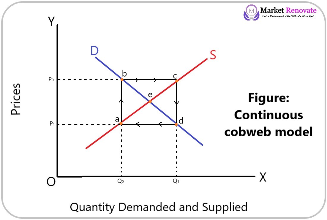
Assume the current year’s price is OP_o, resulting in an OQ₁ supply quantity. This output can be sold at a price of OP₁ in the following period, attracting a demand of OQ₁. However, because the demand exceeds the available supply of OQ_o, the price rises to OP_o = Q₀b.

As a result, prices and quantities will continue to oscillate with constant amplitude around the equilibrium point e.

Implications/ Uses/ Importance of Economic Dynamics:

Economic dynamics is the study of how economic systems change and evolve over time. It encompasses a wide range of economic phenomena, including economic growth and development, business cycles, technological change, and international trade and finance. Economic dynamics is an important field of study, as it helps understand the underlying forces that drive economic change and how they can affect the overall economy.

One of the key implications of economic dynamics is that economic systems are constantly changing and evolving. Economic change can be driven by a wide range of factors, including technological innovations, changes in consumer preferences, shifts in the global economy, and changes in government policies. Economic dynamics help to understand how these factors interact and how they can influence the economy over time.

Another implication of economic dynamics is that economic policy can significantly shape the direction and pace of economic change. Governments and central banks can use tools such as fiscal policy (which involves changes in government spending and taxation) and monetary policy (which involves changes in interest rates and the money supply) to influence the economy. Economic dynamics helps to understand how these policy tools can be used to achieve economic goals, such as promoting growth, stability, or equality.

Similarly, economic dynamics have important implications for businesses and individuals. Economic change can create new opportunities and challenges for businesses, affecting consumers’ availability and cost of goods and services. Understanding economic dynamics can help businesses and individuals make informed decisions about responding to economic change and taking advantage of new opportunities.

Limitation of Economic Dynamics:

Although economic dynamics has provided valuable information into how economic systems change and evolve, it is important to recognize that the field has many limitations.

Based on Simplifying assumptions: Economic dynamics is based on some simplifying assumptions used to simplify economic system analysis. These assumptions may not always hold in the real world and can limit economic models’ accuracy and applicability.
The Complexity of economic systems: Economic systems are complex and multifaceted, and they are influenced by a wide range of factors, including technological innovations, changes in consumer preferences, shifts in the global economy, and changes in government policies. It can be challenging to accurately model and understand the interactions between these factors and how they influence the economy.
Limited data availability: Economic data is often incomplete or imperfect and may not accurately reflect the underlying economic phenomena being studied. This can limit the accuracy and reliability of economic models and analysis.
Forecasting limitations: Economic dynamics are often used to predict future economic trends, but these predictions are subject to high uncertainty. Economic models are based on historic data and are often unable to predict future events or changes in the economy accurately.
Ethical considerations: Economic dynamics often involves making assumptions about human behaviour and decision-making, but these assumptions may not always be accurate or ethical. For example, the assumption that individuals always act in their self-interest may not be consistent with human motivation and decision-making complexity.

Types of Microeconomics or Microeconomic Analysis

Types of Microeconomic Analysis